Context: The Emergence of Big Data

The arrival of big data has introduced significant challenges in data processing, necessitating robust solutions for managing and analyzing massive volumes of information. Conventional single-node processing systems have proven inadequate, leading to the demand for scalable and distributed computing frameworks. In this context, MapReduce has surfaced as a powerful response, providing a framework that efficiently processes and generates large datasets through parallel, distributed algorithms across clusters.

The Mechanics of MapReduce

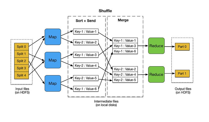
MapReduce is predicated on a straightforward principle: it disaggregates a massive data processing task into smaller, manageable segments, processes them concurrently during the Map step, and subsequently consolidates the outcomes in the Reduce step. This operation consists of two primary phases:

• Map Phase: In this phase, the input dataset is partitioned into smaller subsets. Each subset undergoes a map function, yielding intermediate key-value pairs that simplify the raw data into a more manageable format.
• Reduce Phase: The intermediate key-value pairs generated in the Map phase are grouped, sorted, and shuffled based on shared keys. The reduce function is then applied to each group, merging the associated values to create a smaller set of tuples as the final output.

Application and Versatility

The real strength of MapReduce lies in its flexibility and applicability across a wide range of data processing tasks, from simple counting and sorting to complex data transformations and analyses. It abstracts the underlying complexities of distributed computing, allowing developers to concentrate on mapping and reducing functions without being burdened by infrastructure concerns.

Impact and Evolution

MapReduce has played a crucial role in the growth of big data analytics, enabling the scalable processing of massive datasets. Its integration into the Hadoop ecosystem has further cemented its status as a vital component of contemporary data processing. However, as the field has evolved, MapReduce has faced limitations, including its batch processing nature and inefficiencies in handling fast data and iterative algorithms, which have given rise to more advanced processing models like Apache Spark.

Synthetic Dataset Generation

Initially, we will generate a synthetic dataset that represents sales transactions, complete with product IDs and corresponding sales amounts.

MapReduce Implementation

Next, we will construct a Map function to convert our data into key-value pairs, followed by a Reduce function to aggregate these values based on their keys.

Metrics Calculation

We will compute the total sales for each product and visualize the findings.

Plotting

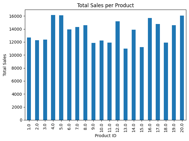
A bar chart will be created to depict total sales per product, offering insights into the data.

import pandas as pd

import numpy as np

import matplotlib.pyplot as plt

# Generate synthetic dataset

np.random.seed(0)

data_size = 1000

product_ids = np.random.randint(1, 21, size=data_size) # 20 products

sales_amounts = np.random.uniform(50, 500, size=data_size)

# Create a DataFrame

df = pd.DataFrame({'Product_ID': product_ids, 'Sales_Amount': sales_amounts})

# MapReduce functions

def map_function(data):

"""Map step: returns a list of key-value pairs (product_id, sales_amount)."""

return [(row['Product_ID'], row['Sales_Amount']) for index, row in data.iterrows()]

def reduce_function(mapped_data):

"""Reduce step: aggregates sales amounts by product_id."""

result = {}

for key, value in mapped_data:

result[key] = result.get(key, 0) + value

return result

# MapReduce execution

mapped_data = map_function(df)

reduced_data = reduce_function(mapped_data)

# Convert reduced data to DataFrame for analysis and plotting

results_df = pd.DataFrame(list(reduced_data.items()), columns=['Product_ID', 'Total_Sales'])

# Plotting

plt.figure(figsize=(10, 6))

results_df.sort_values('Product_ID').plot(kind='bar', x='Product_ID', y='Total_Sales', legend=False)

plt.title('Total Sales per Product')

plt.xlabel('Product ID')

plt.ylabel('Total Sales')

plt.tight_layout()

plt.show()

Interpretation

In this simplified MapReduce illustration, the map function dissects the dataset into key-value pairs of product IDs and sales amounts, simulating the distribution of data processing tasks. The reduce function subsequently aggregates these key-value pairs to compute the total sales per product, mirroring the aggregation phase in MapReduce. The resulting plot visually conveys the total sales per product, exemplifying how MapReduce can be leveraged for aggregating and analyzing large datasets.

The bar chart illustrates total sales per product, where the x-axis denotes Product IDs and the y-axis represents total sales in units. This visualization reveals a relatively even distribution of sales across products, with notable variations. Product ID 3 leads in sales, closely trailed by Product IDs 8 and 6.

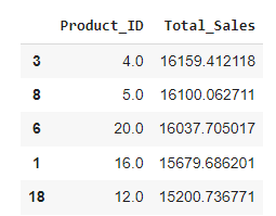
The accompanying table provides a detailed view of the top-selling products, showcasing Product IDs alongside their respective total sales figures. Product ID 3 tops the list with sales of 16,159.41 units, indicating it is the most popular or highest revenue-generating item. Following closely are Product IDs 8, 6, 1, and 18, reflecting strong sales figures ranging from 15,200.74 to 16,159.41 units.

This analysis holds significant implications for business strategy, helping to identify bestsellers, optimize inventory, and refine marketing efforts. Additionally, a balanced sales distribution across products may signify a diversified product strategy that mitigates the risks associated with over-reliance on a single product.